Copula Example

Trying an introduction to copulas exercise, from (R-excerises), using the dataset (https://www.kaggle.com/datasets/gtouzin/samplestocksreturn)

Exercise 1 We’ll start by fitting the margin. First, do a histogram of both Apple and Microsoft returns to see the shape of both distributions.

returns <- read.csv("returns_00_17.csv")
hist(returns$Apple)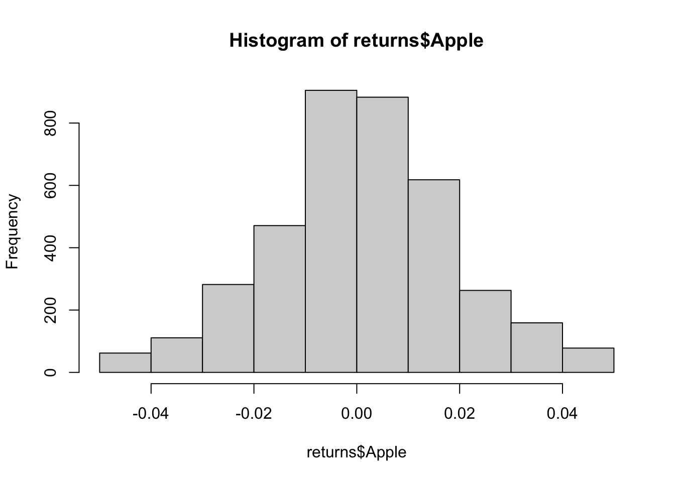

hist(returns$Microsoft)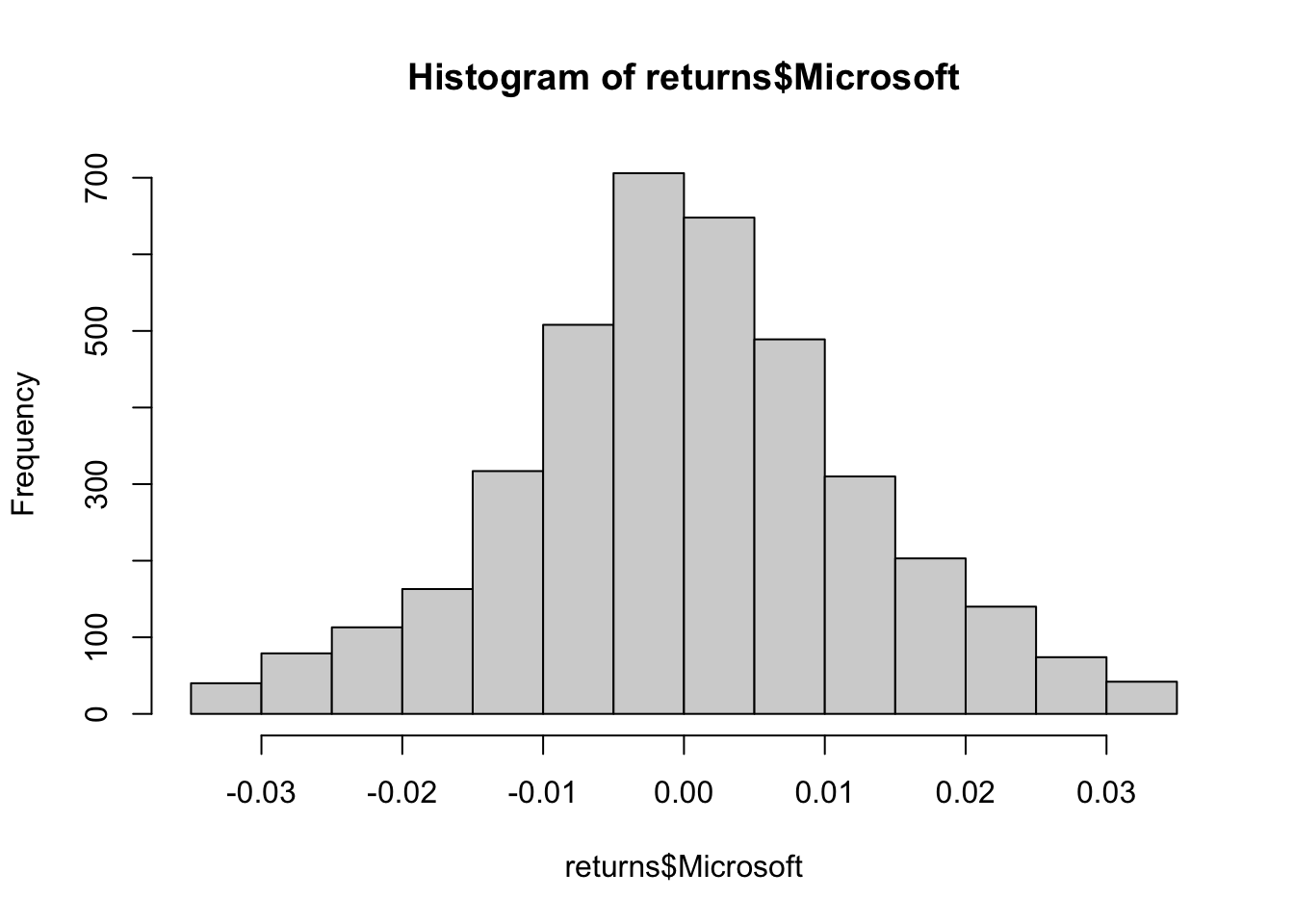

Exercise 2 Both distributions seems symmetric and have a domain which contain positive and negative values. Knowing those facts, use the fitdist() function to see how the normal, logistic and Cauchy distribution fit the Apple returns dataset. Which of those three distributions is best suited to simulate the Apple return dataset and what are the parameter of this distribution?

library(fitdistrplus)

## Loading required package: MASS

## Loading required package: survival

apple.norm <- fitdist(returns$Apple,"norm")
plotdist(returns$Apple,"norm", para=list(mean=apple.norm$estimate[1],sd=apple.norm$estimate[2]))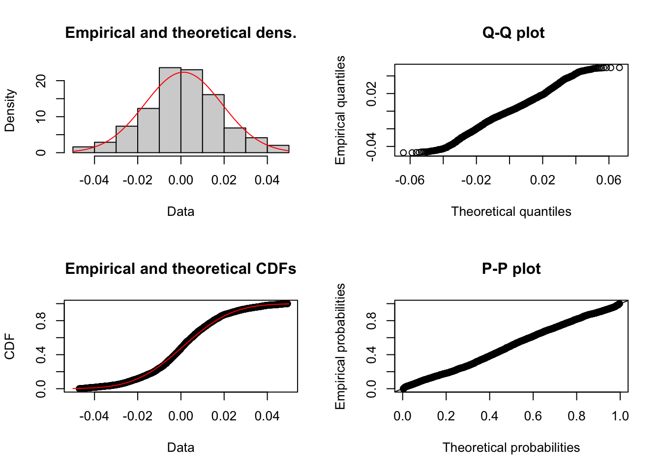

apple.norm$aic

## [1] -19973.54

apple.norm$estimate

##       mean         sd 
## 0.00113756 0.01785252

Exercise 3 Repeat exercise 2 with the Microsoft return.

msft.norm <- fitdist(returns$Microsoft,"norm")
plotdist(returns$Microsoft,"norm", para=list(mean=msft.norm$estimate[1],sd=msft.norm$estimate[2]))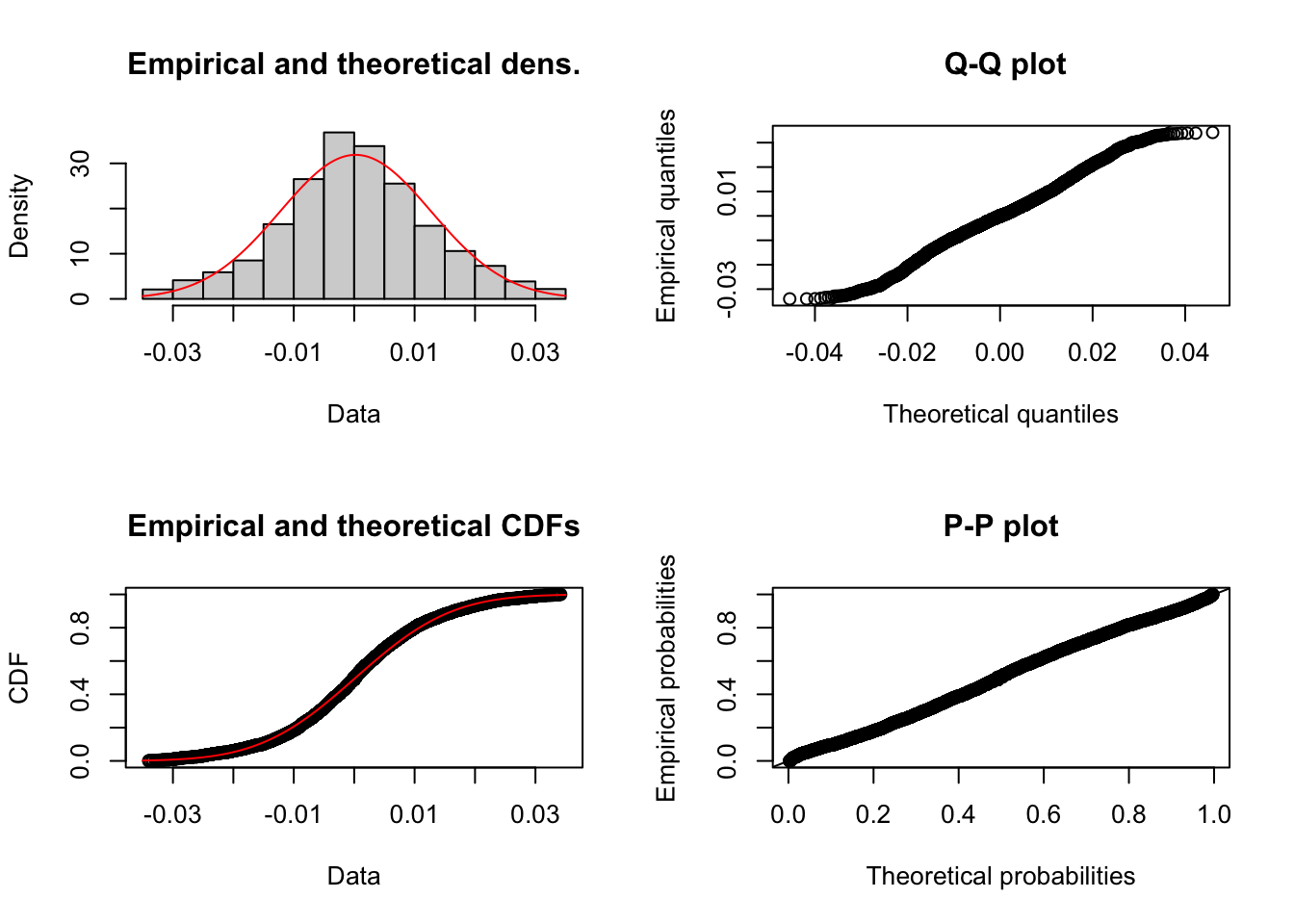

msft.norm$aic

## [1] -22697.15

msft.norm$estimate

##         mean           sd 
## 0.0002408549 0.0125129768

msft.log <- fitdist(returns$Microsoft,"logis")
plotdist(returns$Microsoft,"logis",para=list(location=msft.log$estimate[1],scale=msft.log$estimate[2]))

msft.log$aic

## [1] -22687.25

Exercise 4 Plot the joint distribution of the Apple and Microsoft daily returns. Add the regression line to the plot and compute the correlation of both variables.

plot(returns$Apple,returns$Microsoft)
abline(lm(returns$Apple~returns$Microsoft),col="red")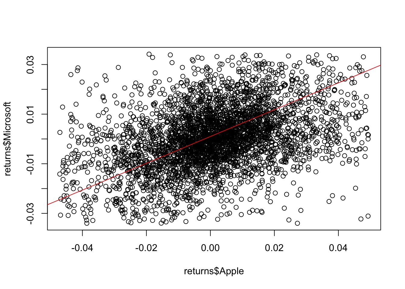

cor(returns$Apple,returns$Microsoft)

## [1] 0.3786614

Exercise 5 Use the pobs() from the VineCopula() package to compute the pseudo-observations for both returns values, then use the BiCopSelect() function to select the copula which minimize the AIC on the dataset. Which copula is selected and what are his parameters.

#install.packages("VineCopula")
library(VineCopula)

x.1 <- pobs(as.matrix(returns[,2:3]))[,1]
x.2 <- pobs(as.matrix(returns[,2:3]))[,2]

apriori.copula <- BiCopSelect(x.1,x.2)

summary(apriori.copula)

## Family
## ------ 
## No:    20
## Name:  Survival BB8
## 
## Parameter(s)
## ------------
## par:  2.55
## par2: 0.77
## Dependence measures
## -------------------
## Kendall's tau:    0.27 (empirical = 0.27, p value < 0.01)
## Upper TD:         0 
## Lower TD:         0 
## 
## Fit statistics
## --------------
## logLik:  335.41 
## AIC:    -666.82 
## BIC:    -654.32

Learn more about MultiVariate analysis in the online course Case Studies in Data Mining with R. In this course you will work thru a case study related to multivariate analysis and how to work with forecasting in the S&P 500.

Exercise 6 Use the appropriate function from the VineCopula() package to create a copula object with the parameter computed in the last exercise. Then, do a three dimensional plot and a contour plot of the copula.

set.seed(42)
bi.cop <- BiCop(20,apriori.copula$par,apriori.copula$par2)

plot(bi.cop, type="contour",size=25,margins="norm")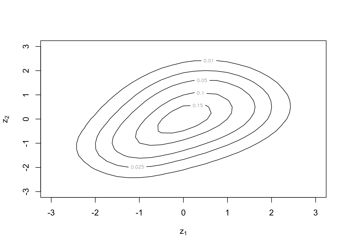

plot(bi.cop, type="surface")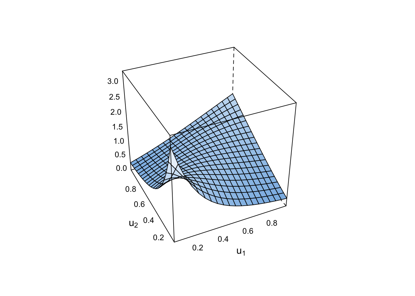

Exercise 7 Set the seed to 42 and generate a sample of 1000 points from this copula. Plot the sample and calculate the correlation of this sample. Does the correlation of the sample is similar to the correlation between the Apple and Microsoft returns?

#install.packages("copula")
library(copula)

## Warning: package 'copula' was built under R version 4.2.3

## 
## Attaching package: 'copula'

## The following object is masked from 'package:VineCopula':
## 
##     pobs

simCopula <- BiCopSim(1000,20,apriori.copula$par,apriori.copula$par2)
plot(simCopula)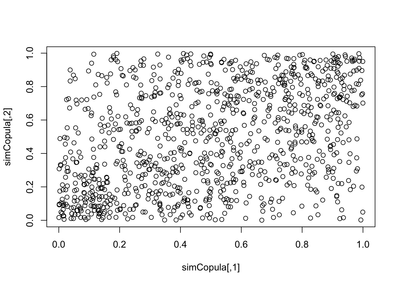

cor(simCopula[,1],simCopula[,2])

## [1] 0.3778374

Exercise 8 Create a distribution from the copula you selected and the margins you fitted in the exercise 2 and 3.

#t.cop <- tCopula(c(0.55,0.77), dim = 2, dispstr = "norm", df = 4,df.fixed = FALSE, df.min = 0.01)

#mjd <- mvdc(copula=t.cop,margins=c("norm","norm"),paramMargins=list(list(mean=apple.norm$estimate[1], sd=apple.norm$estimate[2]),list(mean=msft.norm$estimate[1], sd=msft.norm$estimate[2])))

Exercise 9 Generate 1000 points from the distribution of exercise 8 and plot those points, with the Apple and Microsoft returns, in the same plot.

Exercise 10 Having made a model, let’s make some crude estimation with it! Imagine that this model has been proven to be effective to describe the relation between the apple return and the Microsoft return for a considerable amound of time and there’s a spike in the price of Apple stock. Suppose you have another model who describe the Apple stock and who lead you to believe that the daily return on this stock has a 90% chance to be between 0.038 and 0.045. Using only this information, compute the range containing the possible daily return of the Microsoft stock at the end of the day and the mean of the possible values.

See also