Datacamp’s Tidyverse course using Gapminder dataset
library(gapminder)
library(dplyr)
## Warning: package 'dplyr' was built under R version 4.2.3##
## Attaching package: 'dplyr'## The following objects are masked from 'package:stats':
##
## filter, lag## The following objects are masked from 'package:base':
##
## intersect, setdiff, setequal, unionhead(gapminder)## # A tibble: 6 × 6
## country continent year lifeExp pop gdpPercap
## <fct> <fct> <int> <dbl> <int> <dbl>
## 1 Afghanistan Asia 1952 28.8 8425333 779.
## 2 Afghanistan Asia 1957 30.3 9240934 821.
## 3 Afghanistan Asia 1962 32.0 10267083 853.
## 4 Afghanistan Asia 1967 34.0 11537966 836.
## 5 Afghanistan Asia 1972 36.1 13079460 740.
## 6 Afghanistan Asia 1977 38.4 14880372 786.There are 1706 observations (country, year - pairs)
Using pipes to filter:
gapminder %>%
  filter(year == 2007)
## # A tibble: 142 × 6
## country continent year lifeExp pop gdpPercap
## <fct> <fct> <int> <dbl> <int> <dbl>
## 1 Afghanistan Asia 2007 43.8 31889923 975.
## 2 Albania Europe 2007 76.4 3600523 5937.
## 3 Algeria Africa 2007 72.3 33333216 6223.
## 4 Angola Africa 2007 42.7 12420476 4797.
## 5 Argentina Americas 2007 75.3 40301927 12779.
## 6 Australia Oceania 2007 81.2 20434176 34435.
## 7 Austria Europe 2007 79.8 8199783 36126.
## 8 Bahrain Asia 2007 75.6 708573 29796.
## 9 Bangladesh Asia 2007 64.1 150448339 1391.
## 10 Belgium Europe 2007 79.4 10392226 33693.
## # ℹ 132 more rows142 rows in 2007.
gapminder %>%
  filter(country == "United States", year == 2007)
## # A tibble: 1 × 6
## country continent year lifeExp pop gdpPercap
## <fct> <fct> <int> <dbl> <int> <dbl>
## 1 United States Americas 2007 78.2 301139947 42952.Arrange function.
gapminder %>%
  filter(year == 2007) %>%
  arrange(desc(gdpPercap))
## # A tibble: 142 × 6
## country continent year lifeExp pop gdpPercap
## <fct> <fct> <int> <dbl> <int> <dbl>
## 1 Norway Europe 2007 80.2 4627926 49357.
## 2 Kuwait Asia 2007 77.6 2505559 47307.
## 3 Singapore Asia 2007 80.0 4553009 47143.
## 4 United States Americas 2007 78.2 301139947 42952.
## 5 Ireland Europe 2007 78.9 4109086 40676.
## 6 Hong Kong, China Asia 2007 82.2 6980412 39725.
## 7 Switzerland Europe 2007 81.7 7554661 37506.
## 8 Netherlands Europe 2007 79.8 16570613 36798.
## 9 Canada Americas 2007 80.7 33390141 36319.
## 10 Iceland Europe 2007 81.8 301931 36181.
## # ℹ 132 more rowsMutate function.
gapminder %>%
  mutate(pop = pop / 1000000)
## # A tibble: 1,704 × 6
## country continent year lifeExp pop gdpPercap
## <fct> <fct> <int> <dbl> <dbl> <dbl>
## 1 Afghanistan Asia 1952 28.8 8.43 779.
## 2 Afghanistan Asia 1957 30.3 9.24 821.
## 3 Afghanistan Asia 1962 32.0 10.3 853.
## 4 Afghanistan Asia 1967 34.0 11.5 836.
## 5 Afghanistan Asia 1972 36.1 13.1 740.
## 6 Afghanistan Asia 1977 38.4 14.9 786.
## 7 Afghanistan Asia 1982 39.9 12.9 978.
## 8 Afghanistan Asia 1987 40.8 13.9 852.
## 9 Afghanistan Asia 1992 41.7 16.3 649.
## 10 Afghanistan Asia 1997 41.8 22.2 635.
## # ℹ 1,694 more rowsgapminder %>%
mutate(gdp = gdpPercap * pop)## # A tibble: 1,704 × 7
## country continent year lifeExp pop gdpPercap gdp
## <fct> <fct> <int> <dbl> <int> <dbl> <dbl>
## 1 Afghanistan Asia 1952 28.8 8425333 779. 6567086330.
## 2 Afghanistan Asia 1957 30.3 9240934 821. 7585448670.
## 3 Afghanistan Asia 1962 32.0 10267083 853. 8758855797.
## 4 Afghanistan Asia 1967 34.0 11537966 836. 9648014150.
## 5 Afghanistan Asia 1972 36.1 13079460 740. 9678553274.
## 6 Afghanistan Asia 1977 38.4 14880372 786. 11697659231.
## 7 Afghanistan Asia 1982 39.9 12881816 978. 12598563401.
## 8 Afghanistan Asia 1987 40.8 13867957 852. 11820990309.
## 9 Afghanistan Asia 1992 41.7 16317921 649. 10595901589.
## 10 Afghanistan Asia 1997 41.8 22227415 635. 14121995875.
## # ℹ 1,694 more rowsCombining verbs
gapminder %>%
mutate(gdp = gdpPercap * pop) %>%
filter(year == 2007) %>%
arrange(desc(gdp))## # A tibble: 142 × 7
## country continent year lifeExp pop gdpPercap gdp
## <fct> <fct> <int> <dbl> <int> <dbl> <dbl>
## 1 United States Americas 2007 78.2 301139947 42952. 1.29e13
## 2 China Asia 2007 73.0 1318683096 4959. 6.54e12
## 3 Japan Asia 2007 82.6 127467972 31656. 4.04e12
## 4 India Asia 2007 64.7 1110396331 2452. 2.72e12
## 5 Germany Europe 2007 79.4 82400996 32170. 2.65e12
## 6 United Kingdom Europe 2007 79.4 60776238 33203. 2.02e12
## 7 France Europe 2007 80.7 61083916 30470. 1.86e12
## 8 Brazil Americas 2007 72.4 190010647 9066. 1.72e12
## 9 Italy Europe 2007 80.5 58147733 28570. 1.66e12
## 10 Mexico Americas 2007 76.2 108700891 11978. 1.30e12
## # ℹ 132 more rowsgapminder %>%
filter(year == 2007) %>%
mutate(lifeExpMonths = 12 * lifeExp) %>%
arrange(desc(lifeExpMonths))## # A tibble: 142 × 7
## country continent year lifeExp pop gdpPercap lifeExpMonths
## <fct> <fct> <int> <dbl> <int> <dbl> <dbl>
## 1 Japan Asia 2007 82.6 127467972 31656. 991.
## 2 Hong Kong, China Asia 2007 82.2 6980412 39725. 986.
## 3 Iceland Europe 2007 81.8 301931 36181. 981.
## 4 Switzerland Europe 2007 81.7 7554661 37506. 980.
## 5 Australia Oceania 2007 81.2 20434176 34435. 975.
## 6 Spain Europe 2007 80.9 40448191 28821. 971.
## 7 Sweden Europe 2007 80.9 9031088 33860. 971.
## 8 Israel Asia 2007 80.7 6426679 25523. 969.
## 9 France Europe 2007 80.7 61083916 30470. 968.
## 10 Canada Americas 2007 80.7 33390141 36319. 968.
## # ℹ 132 more rowsggplot2
library(ggplot2)

gapminder_2007 <- gapminder %>% filter(year == 2007)
ggplot(gapminder_2007, aes(x = gdpPercap, y = lifeExp)) +
  geom_point()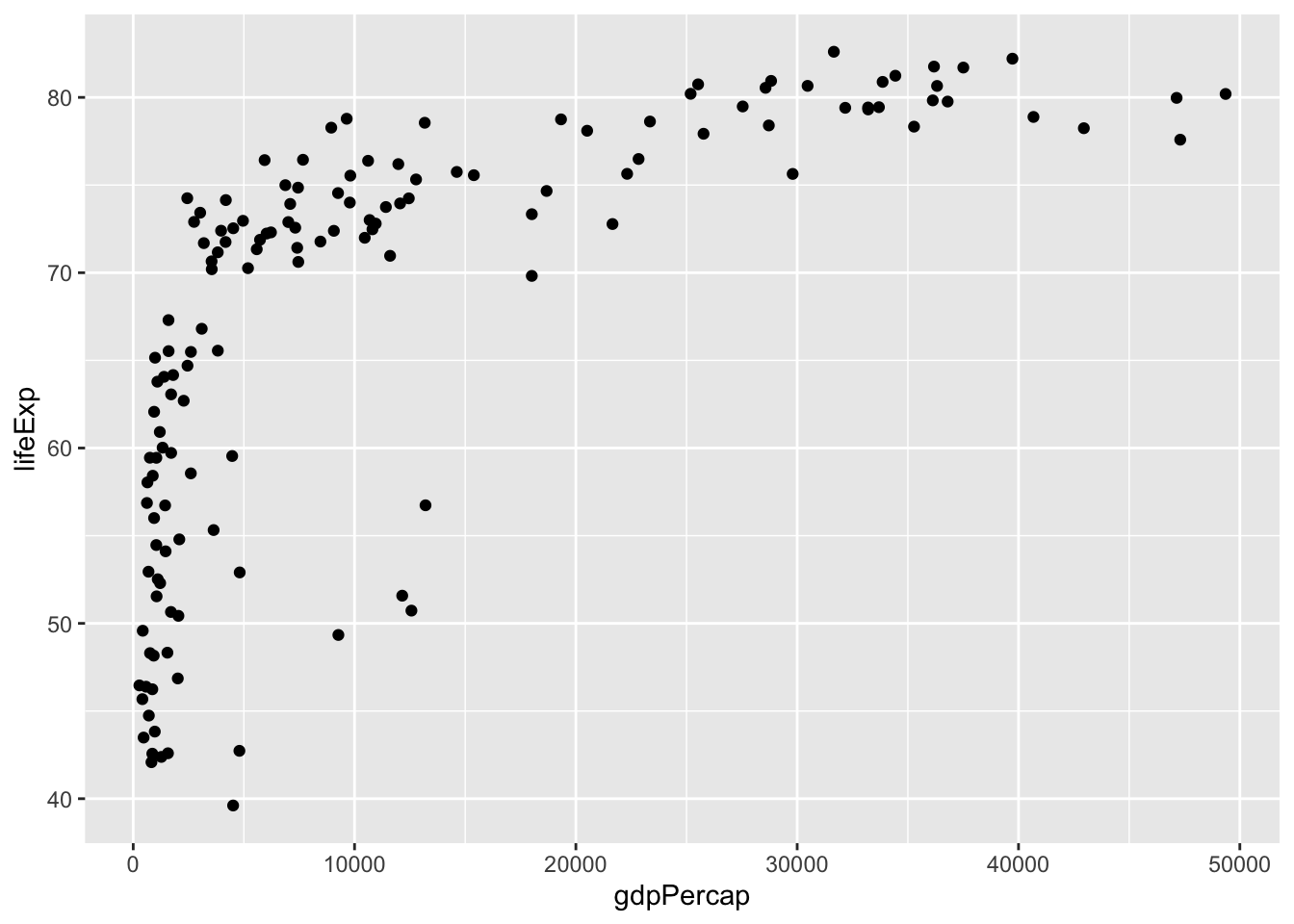
log scale on x-axis
ggplot(gapminder_2007, aes(x = gdpPercap, y = lifeExp)) +
  geom_point() + scale_x_log10()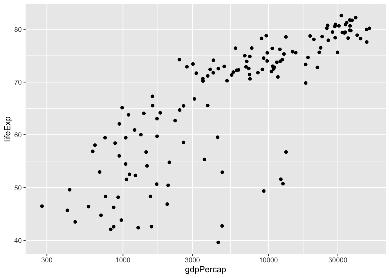
additional aesthetics
ggplot(gapminder_2007,
       aes(
         x = gdpPercap,
         y = lifeExp,
         color = continent,
         size = pop
       )) +
geom_point() + scale_x_log10() 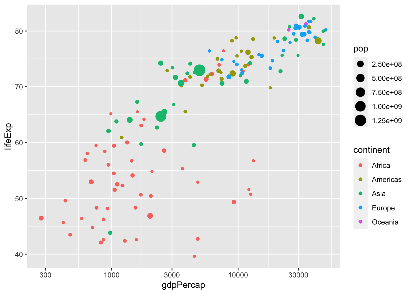
faceting
ggplot(gapminder_2007,
       aes(
         x = gdpPercap,
         y = lifeExp,
         color = continent,
         size = pop
       )) +
  geom_point() + scale_x_log10() + facet_wrap( ~ continent)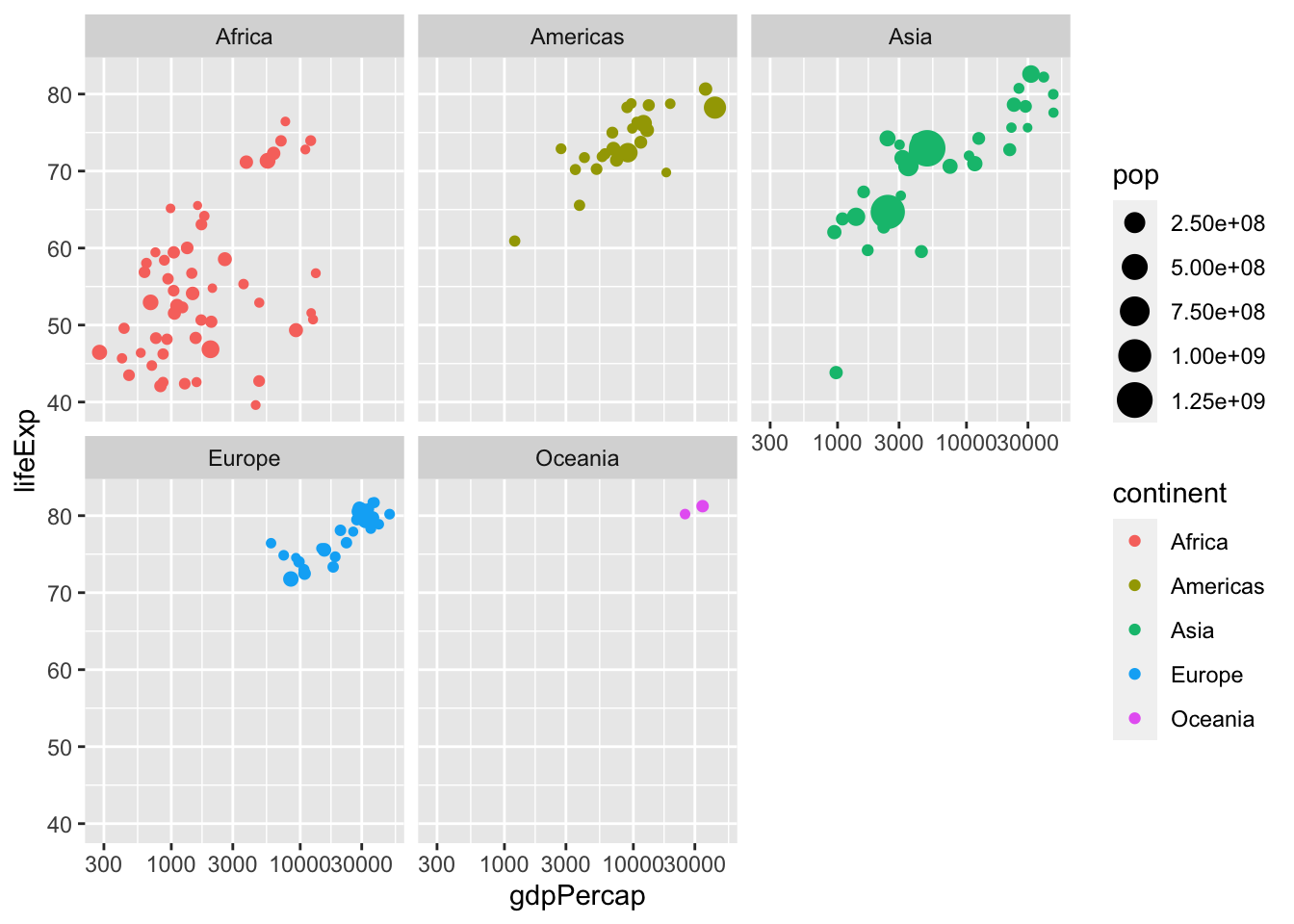
summarize verb
gapminder %>%
  summarize(medianLifeExp = median(lifeExp))
## # A tibble: 1 × 1
## medianLifeExp
## <dbl>
## 1 60.7gapminder %>%
filter(year == 2007) %>%
summarize(meanLifeExp = mean(lifeExp), totalPop = sum(pop))## # A tibble: 1 × 2
## meanLifeExp totalPop
## <dbl> <dbl>
## 1 67.0 6251013179group_by verb
gapminder %>%
  group_by(year, continent) %>%
  summarize(meanLifeExp = mean(lifeExp), totalPop = sum(pop))
## `summarise()` has grouped output by 'year'. You can override using the
## `.groups` argument.## # A tibble: 60 × 4
## # Groups: year [12]
## year continent meanLifeExp totalPop
## <int> <fct> <dbl> <dbl>
## 1 1952 Africa 39.1 237640501
## 2 1952 Americas 53.3 345152446
## 3 1952 Asia 46.3 1395357351
## 4 1952 Europe 64.4 418120846
## 5 1952 Oceania 69.3 10686006
## 6 1957 Africa 41.3 264837738
## 7 1957 Americas 56.0 386953916
## 8 1957 Asia 49.3 1562780599
## 9 1957 Europe 66.7 437890351
## 10 1957 Oceania 70.3 11941976
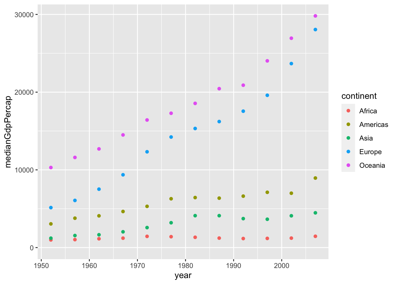
## # ℹ 50 more rows# Summarize medianGdpPercap within each continent within each year: by_year_continent
by_year_continent <- gapminder %>%
group_by(year, continent) %>%
summarize(medianGdpPercap = median(gdpPercap))## `summarise()` has grouped output by 'year'. You can override using the
## `.groups` argument.# Plot the change in medianGdpPercap in each continent over time
ggplot(by_year_continent,
aes(x = year, y = medianGdpPercap, color = continent)) + geom_point() + expand_limits(y = 0)